Load the R packages we will use.
library(tidyverse)
library(moderndive) #install before loading
library(infer) #install before loading
library(fivethirtyeight) #install before loading
Replace all the instances of ???. These are answers on your moodle quiz.
Run all the individual code chunks to make sure the answers in this file correspond with your quiz answers
After you check all your code chunks run then you can knit it. It won’t knit until the ??? are replaced
Save a plot to be your preview plot
Look at the variable definitions in congress_age
What is the average age of members that have served in congress?
Set random seed generator to 123
Take a sample of 100 from the dataset congress_age and assign it to congress_age_100
set.seed(123)
congress_age_100 <- congress_age  %>%
  rep_sample_n(size=100)
congress_age is the population and congress_age_100 is the sample
18,635 is number of observations in the the population and 100 is the number of observations in your sample
Construct the confidence interval
1. Use specify to indicate the variable from congress_age_100 that you are interested in
Response: age (numeric)
# A tibble: 100 x 1
     age
   <dbl>
 1  53.1
 2  54.9
 3  65.3
 4  60.1
 5  43.8
 6  57.9
 7  55.3
 8  46
 9  42.1
10  37
# ... with 90 more rows
2. generate 1000 replicates of your sample of 100
Response: age (numeric)
# A tibble: 100,000 x 2
# Groups:   replicate [1,000]
   replicate   age
       <int> <dbl>
 1         1  42.1
 2         1  71.2
 3         1  45.6
 4         1  39.6
 5         1  56.8
 6         1  71.6
 7         1  60.5
 8         1  56.4
 9         1  43.3
10         1  53.1
# ... with 99,990 more rows
The output has 100,000 rows
3. calculate the mean for each replicate
Assign to bootstrap_distribution_mean_age
Display bootstrap_distribution_mean_age
bootstrap_distribution_mean_age  <- congress_age_100  %>%
  specify(response = age)  %>%
  generate(reps = 1000, type = "bootstrap")  %>%
  calculate(stat = "mean")

bootstrap_distribution_mean_age
Response: age (numeric)
# A tibble: 1,000 x 2
   replicate  stat
       <int> <dbl>
 1         1  53.6
 2         2  53.2
 3         3  52.8
 4         4  51.5
 5         5  53.0
 6         6  54.2
 7         7  52.0
 8         8  52.8
 9         9  53.8
10        10  52.4
# ... with 990 more rows
The bootstrap_distribution_mean_age has 1000 means
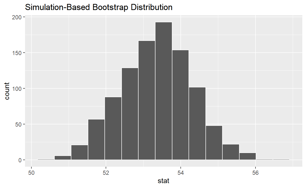
4. visualize the bootstrap distribution
visualize(bootstrap_distribution_mean_age)
Calculate the 95% confidence interval using the percentile method
Assign the output to congress_ci_percentile
Display congress_ci_percentile
congress_ci_percentile  <- bootstrap_distribution_mean_age %>%
  get_confidence_interval(type = "percentile", level = 0.95)

congress_ci_percentile
# A tibble: 1 x 2
  lower_ci upper_ci
     <dbl>    <dbl>
1     51.5     55.2
Calculate the observed point estimate of the mean and assign it to obs_mean_age
Display obs_mean_age
obs_mean_age  <-  congress_age_100  %>%
  specify(response = age)  %>%
  calculate(stat = "mean")  %>%
  pull()

obs_mean_age
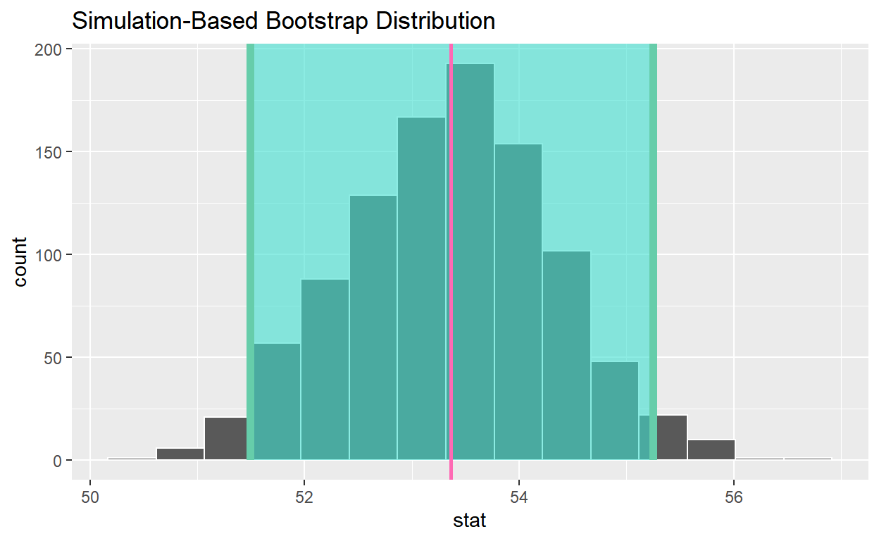
[1] 53.36Shade the confidence interval
Add a line at the observed mean, obs_mean_age, to your visualization and color it “hotpink”
visualize(bootstrap_distribution_mean_age) +
  shade_confidence_interval(endpoints = congress_ci_percentile) +
  geom_vline(xintercept = obs_mean_age, color = "hotpink", size = 1 )
Calculate the population mean to see if it is in the 95% confidence interval
Assign the output to pop_mean_age
Display pop_mean_age
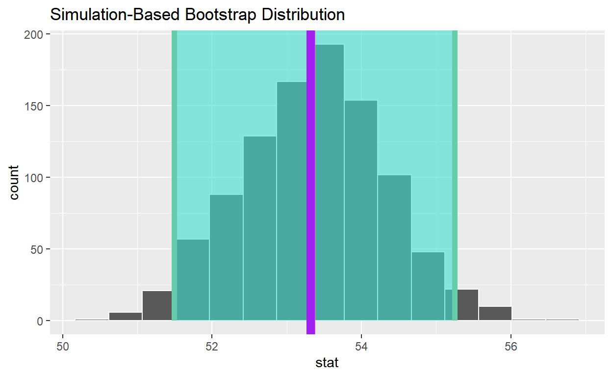
[1] 53.31373- Add a line to the visualization at the, population mean, pop_mean_age, to the plot color it “purple”
visualize(bootstrap_distribution_mean_age) +
  shade_confidence_interval(endpoints = congress_ci_percentile) +
   geom_vline(xintercept = obs_mean_age, color = "hotpink", size = 1) +
   geom_vline(xintercept = pop_mean_age, color = "purple", size = 3)
Save the previous plot to preview.png and add to the yaml chunk at the top
Is population mean the 95% confidence interval constructed using the bootstrap distribution? Yes
Change set.seed(123) to set.seed(4346). Rerun all the code.
When you change the seed is the population mean in the 95% confidence interval constructed using the bootstrap distribution? No
If you construct 100 95% confidence intervals approximately how many do you expect will contain the population mean? 95